This session and the next are about turning a survey file into something you can analyse. That sounds like a chore, and it is the part of the work that textbooks skip. It is also where most of the time goes and where most of the mistakes are made. The analysis itself is usually one or two lines. Everything else is preparation.
This week we do it with base R — the functions that come with R itself. Next week we do the same job with the tidyverse, which is shorter to write. Learning base R first is not a detour: it is what everything else is built on, it is what you will find in older code and in help pages, and it makes clear what the tidyverse is doing for you.
2.1 The data
We use the Swedish study from CSES Module 6, the survey run after the September 2022 general election. The front page of these materials describes it and tells you how to cite it.
There are two files, and the difference matters.
cses6_swe_raw.csv — the survey as it comes. Variable names are CSES codes like F3020_R, and refusals and non-answers are coded as numbers, not as missing.
swe.rds — the cleaned version we use from session 4 onwards.
This week and next we work on the first one and build the second.
2.1.1 Getting the files onto your computer
Every file the course uses is listed on the front page of these materials, under The files. You can also go straight to the two you need this week:
codebook.csv — every variable, what it is, and how it is coded
Click a link and your browser offers to save the file. Two things go wrong here often enough to be worth naming.
A .csv file is plain text, so some browsers show its contents in a new tab instead of saving it. If that happens, go back and right-click the link, then choose “Save link as…”. Do not select the text in the browser window and paste it into a new file. That loses the encoding of the Swedish characters, and the last section of this chapter shows you what a broken encoding costs.
The other is simply that the file lands in Downloads, because that is where browsers put things. It is not where R will look for it.
2.1.2 Where the file goes
In session 1 you made an RStudio Project for this course with a data folder inside it. That folder is where data files belong:
QM/                      the project folder
  QM.Rproj               opening this sets the working directory
  data/
    cses6_swe_raw.csv    move the downloaded file here
    codebook.csv
Move the file out of Downloads and into data. Every path in these materials is written on the assumption that it is there. When you read read.csv("data/cses6_swe_raw.csv") further down this page, it means: the file called cses6_swe_raw.csv, in the folder called data, inside the folder R is working in.
That last part is why the project matters. Open the project by double-clicking QM.Rproj, and R is working in the project folder, so data/ means the right thing. Open the script some other way and it will not.
list.files() shows what is in a folder. Give it the folder name in quotation marks:
If the file you just moved is in that list, you are ready.
If R answers character(0), the folder exists but is empty — the file is still in Downloads. If you get a warning instead, there is no data folder in the place R is looking, which usually means the project is not open.
2.1.3 When R cannot find the file
This is the error you will meet if the file is in the wrong place, and it is worth reading properly once so that you recognise it later:
raw <-read.csv("data/cses6_swe_raw.csv")
Error in file(file, "rt") : cannot open the connection
In addition: Warning message:
In file(file, "rt") :
  cannot open file 'data/cses6_swe_raw.csv': No such file or directory
The first line is R being vague. The useful part is the last one: No such file or directory. R looked for that path and there was nothing there. It is not a problem with your code, and re-running it will not help. There are only three causes, and they are worth checking in this order: the project is not open, the file is still in Downloads, or the name is not quite right — cses_swe_raw.csv and cses6_swe_raw.csv look identical when you are tired.
2.1.4 Letting R do the downloading
You can also have R fetch the files. This takes longer to set up the first time and is worth it, because it makes the work reproducible: someone else can run your script and get the same data without being told where to click.
dir.create() makes a folder. Its showWarnings argument controls whether it complains when the folder is already there, and FALSE means it stays quiet, so the line is safe to run twice.
dir.create("data", showWarnings =FALSE)
download.file() fetches one file. url is the address, destfile is the path to save it to, and mode says how to write it. "wb" means write it as binary — an exact copy of what came down the wire. On macOS and Linux it changes nothing, but on Windows the default alters anything that is not plain text and quietly ruins .rds and .sav files, so write "wb" and it is right everywhere.
Every file on the front page has an address of that shape: the same beginning, then the file name.
One thing you do not need to download: the swirl lessons carry their own copy of the data, so the practical at the end of the chapter works whether or not you have done any of this. The files above are for your own scripts.
2.2 Reading the data into R
2.2.1 R’s own format
R has its own file format, with the extension .rds. It is the most convenient option when you are moving data between your own R sessions, because it stores the object exactly as it was — factors stay factors, and nothing has to be guessed on the way back in.
saveRDS() writes one, and readRDS() reads it. The first argument is the object, and file is where to put it.
Note the pattern on the way back in: readRDS() gives you the object and you have to assign it to a name yourself.
2.2.2 CSV files
The format that works between all software is comma separated values, .csv. It is a plain text file: one line per row, and values within a row separated by commas. You can open one in a text editor and read it, which is exactly why it survives.
read.csv() reads one.
raw <-read.csv("data/cses6_swe_raw.csv")
Three arguments are worth knowing about even though the defaults are usually right.
sep is the character that separates values. The default is a comma. Some countries use a comma as the decimal separator and then a semicolon for the fields, in which case you need sep = ";".
header says whether the first row holds variable names. The default is TRUE.
stringsAsFactors says whether text columns should be turned into factors. Since R 4.0 the default is FALSE, which is what you want. Older code often sets it explicitly, because the default used to be the other way round and it caused a great deal of trouble.
Writing one back out is write.csv(). The row.names argument controls whether the row numbers become a first column; you almost always want FALSE, otherwise every save adds another column of numbers.
SPSS files carry labels: text descriptions attached to the variables and to individual values. haven keeps them, which means the columns come back with a type you have not seen before.
class(raw_spss$F3020_R)
## [1] "numeric"
A haven_labelled vector is a set of numbers with a dictionary attached. That is useful for reading and awkward for computing: some functions will refuse to work with it, and others will quietly do something odd.
attr(raw_spss$F3020_R, "label")
## [1] "Left-right: self"
attr() retrieves an attribute — a piece of information attached to an object without being part of its values. The second argument is which attribute you want.
When you want the numbers and nothing else, zap_labels() strips the labels off.
lr <-zap_labels(raw_spss$F3020_R)class(lr)
## [1] "numeric"
Two functions with similar names do different things, and it is worth keeping them straight. read_sav() from haven keeps the labels. read.spss() from the older foreign package does not, and is fussier. Use haven.
For the rest of this chapter we work with the CSV version, raw, which is plain numbers throughout.
2.3 A first look
Never start analysing a data set you have not looked at. Four functions, in the order you should use them.
dim() gives the size, rows first and columns second.
The [1:12] at the end shows only the first twelve, because all 84 at once is a wall of text. 1:12 builds the sequence of whole numbers from 1 to 12, and the square brackets take those positions.
head() shows the first few rows. Its second argument, n, says how many; the default is 6.
head(raw[, c("F2001_A", "F2002", "F3020_R")], n =4)
Here the square brackets do two things at once. The row position before the comma is empty, so all rows. The column position after the comma is a vector of three names built with c(), so those three columns. The result is a small data frame with everything else left out — which is how you look at a wide data set without drowning.
summary() gives a numerical summary of every column.
##     F2001_A          F3020_R         F3007_1
##  Min.   : 18.00   Min.   : 0.00   Min.   :1.000
##  1st Qu.: 42.00   1st Qu.: 3.00   1st Qu.:2.000
##  Median : 58.00   Median : 6.00   Median :2.000
##  Mean   : 56.13   Mean   :18.32   Mean   :2.321
##  3rd Qu.: 71.00   3rd Qu.: 8.00   3rd Qu.:3.000
##  Max.   :102.00   Max.   :99.00   Max.   :9.000
Now look at that output properly, because two of those three columns are lying to you.
F2001_A is age in years, F3020_R is a left–right self-placement running from 0 to 10, and F3007_1 is trust in parliament running from 1 to 4.
A question. Three things in that output deserve a second look.
The oldest respondent is 102.
Trust in parliament, on a four-point scale, has a maximum of 9.
Left–right self-placement, on a scale from 0 to 10, has a mean of 18.32.
One of these is fine. Two of them are impossible. Which is which, and how do you know without looking anything up?
The third one is the sharpest: a mean can never fall outside the range of the values it is a mean of. What must therefore be true about the values?
That last point is worth holding on to. We did not need the codebook, or the data, to know that something was wrong — only the limits of the scale. Which brings us to the next section.
2.4 What a number stands for
Before going further it is worth being explicit about something that gets skipped. A variable in a data set is a column of numbers. But the numbers are not the point — they stand for something, and what they stand for decides what you are allowed to do with them.
2.4.1 Scales of measurement
The standard division:
Categorical
Binary — two categories. Voted or did not.
Nominal — unordered categories. Which party you voted for.
Ordinal — ordered categories, but the gaps between them are not necessarily equal. “Trust a lot / somewhat / not very much / not at all.”
Continuous
Interval — equal gaps all along the scale, but the zero point is arbitrary. Temperature in Celsius.
Ratio — equal gaps and a real zero, so ratios mean something. Age, income, number of seats.
The practical importance is that the scale decides the method. A mean of a nominal variable is nonsense — the average of “Green party” and “Moderates” does not exist, no matter that both are stored as numbers.
The rule we use in this course. An ordinal variable with five or more categories, numbered at equal intervals, may be treated as continuous. With four or fewer, it may not.
This is a convention rather than a law, and it is not universally agreed. But it is applied consistently throughout these materials, and where an exception is made it is stated and argued for.
2.4.2 Limits
Here is the part that is usually left out, and it is the part that will matter most later.
Every scale has limits, and knowing them is not a technicality — it is most of what you know about a variable before you have looked at any data.
Some limits are hard. They cannot be crossed, because of what the thing is:
A share cannot be below 0% or above 100%.
A count cannot be negative.
A left–right self-placement on a 0-to-10 scale cannot be 11.
A probability lies between 0 and 1.
Some limits are soft. They can in principle be crossed, but effectively are not:
Human age has a hard floor at 0 and a soft ceiling somewhere above 110.
The number of parties winning seats in a district has a hard floor of 1 and a soft ceiling at the number of seats available.
Two things follow, and we use both.
First, limits let you check your work. If a calculation gives a share of 140%, or a probability of −0.2, you do not need to check the data to know something is wrong. The result left the region where answers can exist. We come back to this at the end of the chapter, and every time we compute anything from here on.
Second, limits are the beginning of a model. If you know that a relationship must pass through the point where both variables are zero, and that neither can exceed 100, you already know a great deal about what shape it can have — before collecting a single observation. That is the subject of session 5, and it is worth knowing now that the groundwork is being laid here.
A question. For each of these, what are the limits, and are they hard or soft?
The percentage of women in a parliament.
The difference between how much you like one party and how much you like another, when both are rated 0 to 10.
The number of days per week someone reads the news.
Turnout in an election.
2.5 Looking at one variable
For a categorical variable, table() counts how many cases fall in each category.
table(raw$F3001)
##
##    1    2    3    4    9
##  445 1421  823   90   66
F3001 is political interest, and the CSES codebook says it runs 1 = very interested to 4 = not at all interested, with 9 for missing. You can see all five values here, and the 9s are not a fifth level of interest.
table() ignores NA by default. To make it show them, use the useNA argument:
table(raw$F3001, useNA ="ifany")
##
##    1    2    3    4    9
##  445 1421  823   90   66
"ifany" shows a missing-value column only when there are some. There are none here, and that is exactly the problem: the missing values are still coded as 9.
For a continuous variable, the individual functions are named as you would expect.
mean(raw$F3020_R)
## [1] 18.32056
median(raw$F3020_R)
## [1] 6
sd(raw$F3020_R)
## [1] 32.59899
sd() is the standard deviation. All three of these numbers are wrong, for the same reason as before.
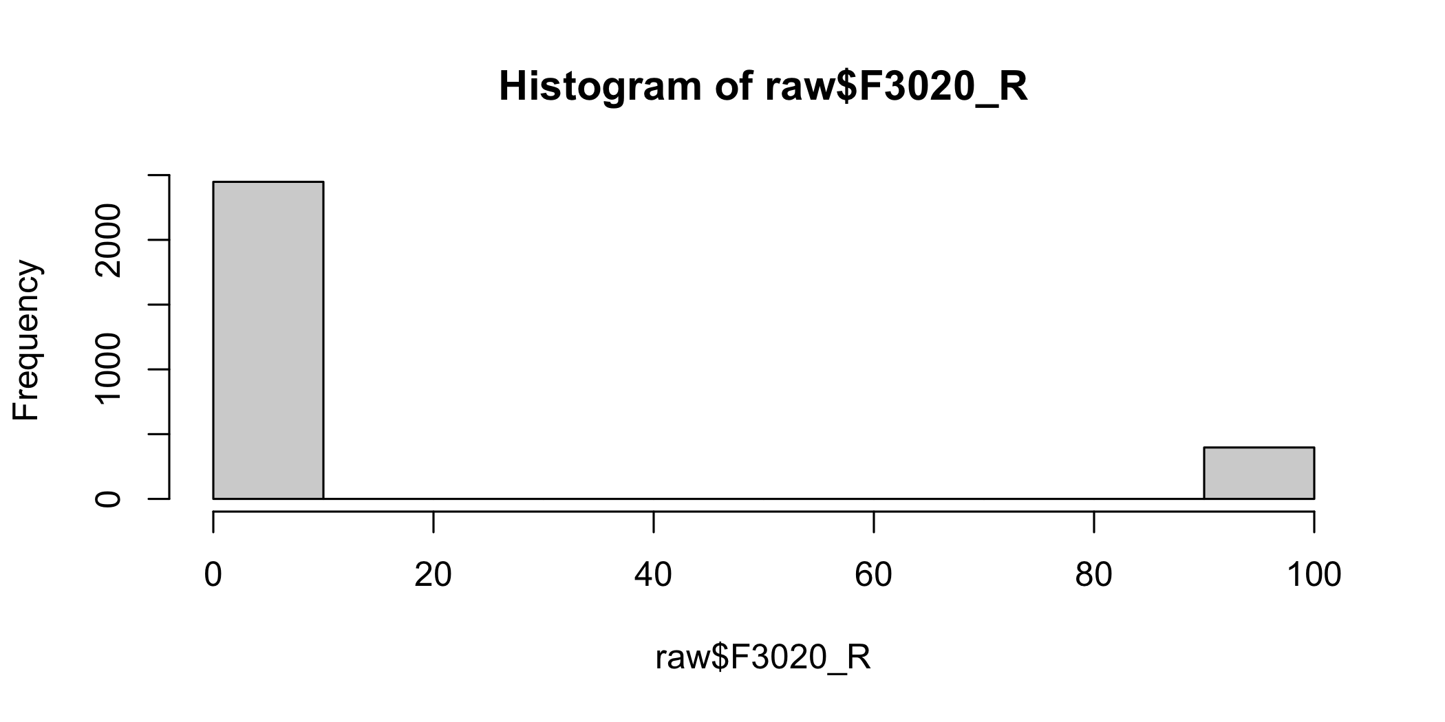
hist() draws a quick histogram. It is not pretty — session 4 is about making plots properly — but it is one word and it shows you the shape.
hist(raw$F3020_R)
The bar at the far right is not a group of extremely right-wing respondents. It is everybody who did not answer.
2.6 Missing values
In R a missing value is NA. In a survey file downloaded from an archive, missing values are usually numbers — and that is the single most dangerous thing about survey data, because nothing warns you.
CSES uses a consistent scheme. On a scale that runs 1 to 4, the codes are 7 for refused, 8 for don’t know, 9 for missing. On a scale that runs 0 to 10, they are 97, 98 and 99. On a variable holding a country code, 997, 998 and 999.
Left in place, they are treated as real answers. A mean of political interest that includes a handful of 9s on a 1-to-4 scale is not slightly wrong; it is wrong in a way that no amount of later care will fix.
2.6.1 Setting them to NA
The tool is the same square-bracket selection you already know, used on the left of an assignment.
Read that middle line from the inside out. polint %in% c(7, 8, 9) asks, for every element of polint, whether it appears in the vector c(7, 8, 9), and gives back TRUE or FALSE for each. Putting that inside square brackets selects the elements where the answer was TRUE. Assigning NA to that selection replaces exactly those.
%in% is worth knowing well. Without it you would write polint == 7 | polint == 8 | polint == 9, which does the same thing at three times the length.
One thing about that first line, which you should not copy.polint <- raw$F3001 lifts the column out of the data frame and leaves it standing on its own. That is done here so the mechanics fit into two lines, and it is a bad habit. A loose vector has lost its connection to the rows it came from: filter or sort the data frame afterwards, or drop a case, and the vector no longer lines up with it. Nothing warns you, and the result is the same class of silent error as the encoding trap at the end of this chapter.
Do it inside the data frame, as a new column beside the original:
Writing the cleaned values back over raw$F3001 instead is sometimes reasonable, since the missing codes are not information anyone wants to keep. It is still the riskier choice. Once the original is gone you cannot check the recode against what it came from, and if the recode turns out to be wrong the only way back is to read the file in again. A new column costs nothing.
The next chapter does all of this with mutate(), which exists precisely so that a new variable lands in the data frame rather than beside it.
Now the table looks sensible:
table(polint, useNA ="ifany")
## polint
##    1    2    3    4 <NA>
##  445 1421  823   90   66
And so does the mean:
mean(polint, na.rm =TRUE)
## [1] 2.200792
Strictly, political interest has four categories, and the rule two sections above says four is not enough to treat as continuous — so this mean is a breach of it. It is used here only to show what the missing codes were doing to the arithmetic, not as a finding about Swedish political interest. Where the materials break a rule they have stated, they will say so; where they do it silently, tell me.
A question. Before we set the missing codes, mean(raw$F3001) was 2.36. After, it is 2.2.
The scale runs from 1 to 4. Was the first number obviously wrong just by looking at it? What does that tell you about relying on a number looking reasonable?
2.6.2 How much is missing
Count missing values by testing with is.na() and adding up the TRUEs.
sum(is.na(polint))
## [1] 66
As a proportion, mean() of a TRUE/FALSE vector gives the share that are TRUE:
mean(is.na(polint))
## [1] 0.02319859
So about 2.3% missing, which is fine.
complete.cases() tests whole rows, giving TRUE for a row with no missing values anywhere in it. Try it on three of the original columns:
Every single row is complete — all 2 845 of them. That is not good news. It is complete.cases() telling the truth about a data frame in which the missing values have not yet been marked as missing. There is nothing for it to find, because the gaps are still disguised as the numbers 9 and 99.
444 respondents have a gap on at least one of these three variables. That is the number that was there all along.
Watch this number as you add variables to a model. Every variable you add drops every respondent who is missing on it, and the losses compound. A model with ten variables can quietly be fitted on half your sample — and it will not tell you unless you ask.
2.7 Selecting rows and columns
You already know the basic form: [rows, columns].
By position:
raw[3, 1:3]
##   F1003_2    F1004 F1006_NAM
## 3    2341 SWE_2022    Sweden
By name, which is safer, because inserting a column shifts every number:
head(raw[, c("F2002", "F2003")], n =3)
##   F2002 F2003
## 1     0     8
## 2     0     7
## 3     0     6
The useful case is selecting rows by condition. A comparison on a column gives a TRUE/FALSE vector as long as the data frame, and putting that in the row position keeps the TRUE rows.
young <- raw[raw$F2001_A <30, ]dim(young)
## [1] 274 84
Conditions combine with & for “and” and | for “or”.
A trap. Selecting rows this way keeps rows where the condition is NA, and fills them with NA. If F2001_A had missing values coded as NA, raw[raw$F2001_A < 30, ] would give you the young respondents plus a row of NAs for every respondent whose age is unknown — because R does not know whether an unknown age is under 30, so it will not say either way.
The fix is which(), which converts a TRUE/FALSE vector into the positions of the TRUEs, dropping the NAs:
raw[which(raw$F2001_A < 30), ]
Use which() whenever the variable you are testing might have missing values. Next week’s filter() handles this for you, which is one of several reasons to prefer it.
2.8 Recoding
Recoding means making a new variable out of an existing one. Three cases cover almost everything.
Never overwrite the original. Make a new variable. When the recode turns out to be wrong — and it will, at least once — you need the original to go back to. This is also why all of this belongs in a script rather than being done by hand.
2.8.1 Reversing a scale
CSES codes political interest with 1 as most interested. That is backwards for reading results: in a regression, a positive coefficient would mean less interest. Reversing it costs one line.
Why 5? For a scale running from lo to hi, the reversed value is (hi + lo) - x. Here that is 4 + 1 = 5. Check it against the table: the 1s and the 4s have swapped, and so have the 2s and 3s, and the total count is unchanged.
That last sentence is the important habit. A recode is a claim, and a claim can be checked. Comparing the before and after tables takes five seconds and catches the error that would otherwise survive into your results.
2.8.2 Grouping a continuous variable
Suppose we want age in three groups. Start by creating a variable that is entirely missing, then fill it in.
age <- raw$F2001_Aage[age %in%c(9997, 9998, 9999)] <-NArange(age, na.rm =TRUE)
## [1] 18 102
As it happens the Swedish study has no missing ages at all, so that second line changed nothing — the range runs from 18 to 102. Write it anyway. You do not know a variable has no missing codes until you have checked, and a line that does nothing costs nothing.
The oldest respondent being 102 is the answer to part of the earlier question: age has a hard floor and only a soft ceiling, and 102 is on the right side of it. Unusual is not the same as impossible.
agegroup <-rep(NA, length(age))agegroup[which(age <35)] <-"Under 35"agegroup[which(age >=35& age <65)] <-"35 to 64"agegroup[which(age >=65)] <-"65 and over"
rep() repeats a value; here it makes a vector of NA the same length as age. length() gives the number of elements.
Starting from all-missing is deliberate. Anything the conditions fail to cover stays NA rather than silently taking a wrong value — so if the conditions have a gap, you find out.
Note which() again, for the reason given above: age has missing values.
table(agegroup, useNA ="ifany")
## agegroup
##    35 to 64 65 and over    Under 35
##        1332        1066         447
The counts add up to 2 845, which is every respondent, and no category is empty. Had a respondent fallen through the conditions — an age of exactly 35 slipping between two of them, say — they would be sitting in an NA column here, and the total would still add up. That is the check, and it is why we started from all-missing rather than from a default value.
2.8.3 Putting categories in order
There is a problem with that table: the categories are in alphabetical order, so “65 and over” comes before “Under 35”. Alphabetical order is not the order of the variable.
Text becomes an ordered categorical variable when you make it a factor and say what the order is.
agegroup <-factor( agegroup,levels =c("Under 35", "35 to 64", "65 and over"))table(agegroup, useNA ="ifany")
## agegroup
##    Under 35    35 to 64 65 and over
##         447        1332        1066
levels gives the categories in the order you want them. From here on, every table and every plot will use that order.
levels also decides which category is the reference when a factor goes into a regression — the one the others get compared to. That is session 13, but the choice is made here.
2.8.4 Collapsing categories
Merging categories works the same way, with == instead of a range.
Every column has its count in exactly one row, and the row it is in is the one intended. That is what a correct collapse looks like, and it takes one line to confirm.
2.9 Checking your work
This section is short and it is the most important one in the chapter.
Every variable has limits. After a recode, the values must still be inside them. Checking this by eye works until you have sixty variables, at which point it stops working and you do not notice.
So check by machine. range() gives the smallest and largest value; na.rm = TRUE is needed or a single NA makes both of them NA.
range(polint_rev, na.rm =TRUE)
## [1] 1 4
Better still, make the check fail loudly. stopifnot() takes one or more conditions and does nothing at all if they are all TRUE — but stops with an error if any is FALSE.
Nothing printed, which means it passed. Had the recode been wrong, the script would have stopped there rather than carrying the mistake into a model output that looks perfectly plausible.
This is worth the small effort it costs. A wrong number that is obviously wrong is a nuisance. A wrong number that looks reasonable is a problem, because nothing will tell you. The limits of the scale are what let you tell the difference, and they are known before you start.
2.10 A trap worth meeting once
One more thing, because it costs hours when it happens and it gives no error message.
The Swedish county names contain å, ä and ö. Suppose the county names are read from one file, and somewhere in a script you write out "Götaland" to compare against them. Sometimes the comparison fails — even though the two strings look identical and contain exactly the same bytes.
The reason is that R records, alongside the text, which encoding it thinks the text is in. If one string is tagged as UTF-8 and the other is not, R can treat them as different. There is no error and no warning. The comparison simply returns FALSE, and every row that should have matched becomes NA.
This happened while preparing the data for this course, and it silently lost 1,357 of the 2,845 rows. The only visible symptom was a category with a count of zero.
Two habits prevent it:
Where a set of category names exists in a file, take them from the file rather than typing them again in your script.
Pin the encoding at the top of the script, so it does not depend on the machine:
Sys.setlocale("LC_CTYPE", "en_US.UTF-8")
The general lesson is worth more than the specific fix. Errors that produce a message are cheap: you find them immediately. Errors that produce a wrong answer are expensive, and text comparison is one of the places they live.
In the seminar.swirl lesson 02 Data Management I. Reading the survey file, looking at it, dealing with the missing-value codes, subsetting and recoding. Around 30 minutes.
2.11 Appendix: what the variables are
CSES ships its variables under names like F3020_R and F3011_LH_PL. They are not meant to be read. They are positions in a codebook that runs to several hundred pages and covers every country in the study, and working from them directly is how people end up analysing the wrong column without noticing.
So the variables were renamed when the data for this course were built: F3020_R became lr_self, F3007_1 became tr_parl. The table below is the map between the two, and it is the page to come back to whenever you meet a name you do not recognise — in these materials, in a swirl lesson, or in your own work.
The columns are these.
Name — what the variable is called in swe.rds, the cleaned file we use from session 4 onwards.
CSES name — the name the variable has in the archive. This is what you will find in cses6_swe_raw.csv and what you look up in the official CSES codebook.
What it is — what was asked, in one line.
Coding — the values and what they mean, after cleaning. In the raw file the missing-value codes are still there, which is the whole subject of this session.
Sessions — which sessions use the variable.
38 of the 85 variables are used somewhere in the course. A blank in the last column means the variable is in the data set but we never touch it, and those are there deliberately: they are the obvious place to look if you want a question of your own to work on.
The same table is downloadable as codebook.csv, which is easier to search than a web page.
2.11.1 Identifier and weight
Name
CSES name
What it is
Coding
Sessions
id
F1003_2
Respondent identifier
Text
wt
F1101_2
Survey weight
Demographic raking weight (gender, age, education). Mean 1
2.11.2 Who the respondent is
Name
CSES name
What it is
Coding
Sessions
age
F2001_A
Age in years
Years
1, 2, 3, 4, 9, 11, 12, 14
female
F2002
Gender
0 = male, 1 = female
7, 8, 13, 14, 15
educ
F2003
Education
1-9 on the ISCED scale, 9 = doctoral
11, 12, 15
educ3
F2003
Education in three groups
No degree / Bachelor / Postgraduate
4, 7, 13
marital
F2004
Marital status
Married / Widowed / Divorced / Single
union
F2005
Union membership
0 = no, 1 = yes
ses
F2008
Socio-economic status
White collar / Worker / Farmer / Self-employed
7, 8
income
F2010_1
Household income
1 = lowest quintile to 5 = highest
relig
F2012
Attendance at religious services
1 = never to 6 = weekly or more
bornswe
F2015
Born in Sweden
0 = no, 1 = yes
foreignpar
F2016
Was either parent born abroad
0 = no, 1 = yes
urban
F2020
Rural or urban residence
1 = rural to 4 = large town or city
county
F2018
County of residence
One of the 21 Swedish counties
3
land
F2018
Historical land
Götaland / Svealand / Norrland, south to north
3
2.11.3 Politics in general
Name
CSES name
What it is
Coding
Sessions
polint
F3001
Political interest
1 = not at all to 4 = very interested (reversed)
2, 3
inteff
F3003
Internal efficacy
1 = strongly disagree to 5 = strongly agree (reversed)
news_tv
F3002_1
News on public television
Days per week 0-7
news_web
F3002_5
Online news sites
Days per week 0-7
news_soc
F3002_6_1
News on social media
Days per week 0-7
2.11.4 Views on democracy
Name
CSES name
What it is
Coding
Sessions
dem_pref
F3004_1
Democracy is always preferable
1-5, agreement (reversed)
dem_courts
F3004_2
Courts should stop the government
1-5, agreement (reversed)
dem_strong
F3004_3
Strong leader who bends the rules is good
1-5, agreement (reversed)
dem_women
F3004_4
Representation of women has gone too far
1-5, agreement (reversed)
run_business
F3005_1
Country better run by business leaders
1-5, agreement (reversed)
run_experts
F3005_2
Country better run by independent experts
1-5, agreement (reversed)
run_referenda
F3005_3
Country better run by citizens in referendums
1-5, agreement (reversed)
demlevel
F3006
How democratic is the country
0 = not at all to 10 = completely
10, 11, 12, 14
satdem
F3022
Satisfaction with democracy
1 = not at all to 4 = very satisfied (reversed, gap closed)
3, 9, 10
fairgroups
F3026
Are all groups in society treated fairly
1 = not at all to 4 = very fairly (reversed)
health
F3027
Does the system guarantee adequate healthcare
1 = not at all to 4 = very well (reversed)
2.11.5 Trust
Name
CSES name
What it is
Coding
Sessions
tr_parl
F3007_1
Trust in parliament
1 = not at all to 4 = a lot (reversed)
3, 10, 11, 12, 14, 15
tr_govt
F3007_2
Trust in the government
1 = not at all to 4 = a lot (reversed)
9, 10, 11, 12, 14, 15
tr_court
F3007_3
Trust in the judiciary
1 = not at all to 4 = a lot (reversed)
10, 11, 12, 14, 15
tr_sci
F3007_4
Trust in scientists
1 = not at all to 4 = a lot (reversed)
10, 11, 12, 14, 15
tr_party
F3007_5
Trust in political parties
1 = not at all to 4 = a lot (reversed)
10, 11, 12, 14, 15
tr_media
F3007_6
Trust in traditional media
1 = not at all to 4 = a lot (reversed)
10, 11, 12, 14, 15
tr_socmed
F3007_7
Trust in social media
1 = not at all to 4 = a lot (reversed)
10
2.11.6 The government and the economy
Name
CSES name
What it is
Coding
Sessions
govperf
F3008_1
Performance of the government
1 = very bad to 4 = very good (reversed)
govcovid
F3008_2
Performance of the government in the pandemic
1 = very bad to 4 = very good (reversed)
econ
F3009
State of the economy over the past year
1 = much worse to 5 = much better (reversed)
2.11.7 The election
Name
CSES name
What it is
Coding
Sessions
satvote
F3012_1
Satisfaction with own vote
1 = not at all to 4 = very satisfied (reversed, gap closed)
satchoice
F3013
Satisfaction with the choice on offer
1 = not at all to 4 = very satisfied (reversed, gap closed)
fair
F3014
Was the election conducted fairly
1 = unfairly to 5 = fairly (reversed)
exteff
F3017
External efficacy
1 = voting makes no difference to 5 = a big difference
2.11.8 The pandemic
Name
CSES name
What it is
Coding
Sessions
pand_unity
F3028_1
Effect of the pandemic on a united society
1 = very negative to 5 = very positive (reversed)
pand_dem
F3028_2
Effect of the pandemic on democracy
1 = very negative to 5 = very positive (reversed)
pand_fin
F3028_3
Effect of the pandemic on personal finances
1 = very negative to 5 = very positive (reversed)
covid
F3028_4
Anyone in the household had covid-19
0 = no, 1 = yes
2.11.9 How the parties are rated
Name
CSES name
What it is
Coding
Sessions
like_s
F3018_A
Rating of the Social Democrats (S)
0 = strongly dislike to 10 = strongly like
4, 5, 8, 9
like_sd
F3018_B
Rating of the Sweden Democrats (SD)
0 = strongly dislike to 10 = strongly like
5, 8, 9
like_m
F3018_C
Rating of the Moderates (M)
0 = strongly dislike to 10 = strongly like
4, 5, 8, 9
like_v
F3018_D
Rating of the Left Party (V)
0 = strongly dislike to 10 = strongly like
5, 8, 9
like_c
F3018_E
Rating of the Centre Party (C)
0 = strongly dislike to 10 = strongly like
5, 8, 9
like_kd
F3018_F
Rating of the Christian Democrats (KD)
0 = strongly dislike to 10 = strongly like
5, 8, 9
like_mp
F3018_G
Rating of the Greens (MP)
0 = strongly dislike to 10 = strongly like
5, 8, 9
like_l
F3018_H
Rating of the Liberals (L)
0 = strongly dislike to 10 = strongly like
5, 8, 9
2.11.10 How the party leaders are rated
Name
CSES name
What it is
Coding
Sessions
lead_andersson
F3019_A
Rating of Magdalena Andersson (S)
0 = strongly dislike to 10 = strongly like
8
lead_akesson
F3019_B
Rating of Jimmie Åkesson (SD)
0 = strongly dislike to 10 = strongly like
8
lead_kristersson
F3019_C
Rating of Ulf Kristersson (M)
0 = strongly dislike to 10 = strongly like
8
lead_dadgostar
F3019_D
Rating of Nooshi Dadgostar (V)
0 = strongly dislike to 10 = strongly like
8
lead_loof
F3019_E
Rating of Annie Lööf (C)
0 = strongly dislike to 10 = strongly like
8
lead_busch
F3019_F
Rating of Ebba Busch (KD)
0 = strongly dislike to 10 = strongly like
8
lead_stenevi
F3019_G
Rating of Märta Stenevi (MP)
0 = strongly dislike to 10 = strongly like
8
lead_pehrson
F3019_H
Rating of Johan Pehrson (L)
0 = strongly dislike to 10 = strongly like
8
2.11.11 Left and right
Name
CSES name
What it is
Coding
Sessions
lr_s
F3020_A
Social Democrats on the left-right scale
0 = left to 10 = right
lr_sd
F3020_B
Sweden Democrats on the left-right scale
0 = left to 10 = right
lr_m
F3020_C
Moderates on the left-right scale
0 = left to 10 = right
lr_v
F3020_D
Left Party on the left-right scale
0 = left to 10 = right
lr_c
F3020_E
Centre Party on the left-right scale
0 = left to 10 = right
lr_kd
F3020_F
Christian Democrats on the left-right scale
0 = left to 10 = right
lr_mp
F3020_G
Greens on the left-right scale
0 = left to 10 = right
lr_l
F3020_H
Liberals on the left-right scale
0 = left to 10 = right
lr_self
F3020_R
Own place on the left-right scale
0 = left to 10 = right
3, 4, 6, 8, 9, 13, 14, 15
2.11.12 Voting
Name
CSES name
What it is
Coding
Sessions
turnout
F3010
Cast a ballot
0 = no, 1 = yes. Almost no variation
6
vote
F3011_LH_PL
Vote choice
The eight parties, in left-to-right order
1, 3, 4, 5, 6, 7, 10, 13
prevvote
F3016_LH_PL
Vote choice in 2018
The eight parties, in left-to-right order
switched
derived
Voted for a different party than in 2018
0 = no, 1 = yes
bloc
derived
Government-formation bloc in 2022
Left (S, V, MP, C) / Right (M, SD, KD, L)
4, 7, 11, 12, 14
vote_sd
derived
Voted for the Sweden Democrats
0 = no, 1 = yes
7, 15
vote_right
derived
Voted for the right bloc
0 = no, 1 = yes
vote_inc
F3011_OUTGOV
Voted for the incumbent government
0 = no, 1 = yes
pid
F3023_1
Feels close to a party
0 = no, 1 = yes
pid_close
F3023_4
How close to that party
1 = not very to 3 = very close (reversed). Only asked of those who feel close